Cisco CCNA Cyber Ops SECFND 210-250, Section 2: Understanding the Network Infrastructure

2.2 Analyzing DHCP Operations
2.3 IP Subnetting
2.4 Hubs, Bridges, and Layer 2 Switches
2.5 VLANs and Trunks
2.6 Spanning Tree Protocols
2.7 Standalone (Autonomous) and Lightweight Access Points
2.8 Routers
2.9 Routing Protocols
2.10 Multilayer Switches
2.11 NAT Fundamentals
2.12 Packet Filtering with ACLs
2.13 ACLs with the Established Option

Analyzing DHCP Operations
Various attacks are emerging that target the Dynamic Host Configuration Protocol or DHCP. In any organization with multiple DHCP clients, DHCP server availability is critical. It is important for security analysts to understand the DHCP messages that are exchanged between the DHCP server and the DHCP client, in order to effectively monitor, troubleshoot, and mitigate DHCP-based attacks. Moreover, when analyzing logs, identifying or correlating attack-related issues is easier for the security analyst who has a solid understanding of DHCP and how it functions.

In large environments, manual address assignment can become an excessive administrative problem, especially for mobile devices that roam from one network to another many times each day. DHCP is a standardized network protocol for dynamically distributing IP addresses automatically, and setting other network configuration parameters, such as the subnet mask, default router, and DNS servers. With DHCP, computers request IP addresses and networking parameters automatically from a DHCP server, reducing the need for network administrators or users to manually configure these settings.

In an enterprise environment, a DHCP server is usually a dedicated device; in smaller deployments or some branch offices, it can be configured on DHCP-capable switches or routers.

DHCP employs a connectionless service model using UDP, and is implemented using the same two UDP port numbers as BOOTP (Bootstrap Protocol). In fact, DHCP is implemented as an option of BOOTP and uses BOOTP as its transport protocol. UDP port number 67 is the destination port of a DHCP server, and UDP port number 68 is used by the DHCP client.

Some of the most common messages that are exchanged between the DHCP server and the client are as follows:

DHCPDISCOVER

DHCPOFFER

DHCPREQUEST

DHCPACK

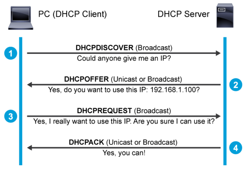
When a computer or other networked device connects to a network, the DHCP client software sends out a DHCPDISCOVER message on its local physical subnet over UDP port 67, which is a broadcast message to locate available servers.

When a DHCP server receives a DHCPDISCOVER message from a client, which is an IP address lease request, the server reserves an IP address for the client and makes a lease offer by sending a DHCPOFFER message to the client on UDP port 68. This message contains the client’s MAC address, the IP address that the server is offering, the subnet mask, the lease duration, and the IP address of the DHCP server that is making the offer. The offer from the DHCP server is not a guarantee that the IP address will be allocated to the client; however, the server usually reserves the address until the client has had a chance to formally request the address.

After the client receives a DHCPOFFER, it responds with a DHCPREQUEST message, indicating its intent to accept the parameters in the DHCPOFFER. A client can receive DHCP offers from multiple servers, but it will accept only one DHCP offer.

When the DHCP server receives the DHCPREQUEST message from the client, the configuration process enters its final phase. The acknowledgement phase involves sending a DHCPACK packet to the client. This packet includes the lease duration and any other configuration information that the client might have requested. At this point, the IP configuration process is completed.


Note:
As indicated in the figure above, DHCPOFFER and DHCPACK messages are sometimes sent as broadcasts instead of unicasts. For details, refer to [RFC 2131](http://www.rfc-editor.org/rfc/rfc2131.txt){:target="_blank"}, Dynamic Host Configuration Protocol.

The lease mechanism ensures that hosts that have been moved or are switched off for extended periods do not keep addresses that they do not use. The addresses are returned to the address pool by the DHCP server, to be reallocated as necessary.

In addition to the four most common DHCP messages, you might also see other DHCP messages in packet captures as follows:

DHCPNAK: A DHCPNAK is a negative acknowledgment from the DHCP server. For example, the server sends DHCPNAK if the client requests an address that is already in use by another client.

DHCPDECLINE: If the DHCP client determines the offered configuration parameters are invalid, it sends a DHCPDECLINE packet to the server, and the client must begin the lease process again.

DHCPRELEASE: After the client is ready to give up the DHCP IP address, it sends a DHCPRELEASE message.

DHCPINFORM: A DHCP client that already has an IP address can use DHCPINFORM message to request more information from the server. For example, browsers use DHCP Inform to obtain web proxy settings.

DHCP Relay Agent
The DHCP server does not have to reside directly on the same subnet where the DHCP client resides. Moreover, it’s impractical to have a DHCP server on every subnet. Most enterprise networks will have a few centralized DHCP servers. The DHCP relay agent acts as an intermediary and ensures that local DHCP client requests are passed onto centralized DHCP servers. Any Layer 3 capable devices such as routers or switches can function as the DHCP relay agent.

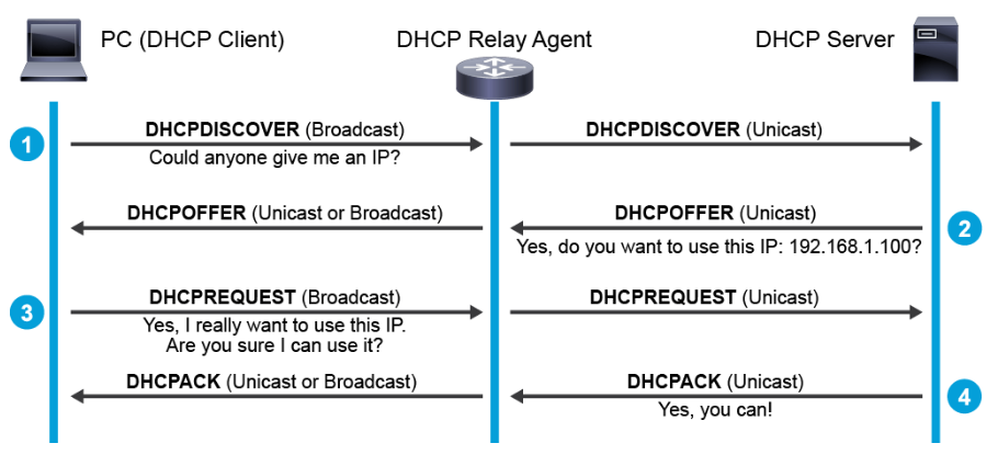
The primary function of a DHCP relay agent is to forward DHCP messages from the local clients to the remote DHCP server.

When a DHCP relay agent receives a broadcast packet from a connected client, it examines the giaddr(Gateway IP Address) field. If the field has an IP address of 0.0.0.0, then the DHCP relay agent changes the giaddr field in DHCP packets from zero to the relay agent IP address and forwards the message to the remote subnet where the DHCP server is located.

The DHCP server uses this IP address to select an IP address pool from which to assign the IP addresses to the DHCP client.

The return packets from the DHCP server are directly sent to the relay agent identified in the giaddr field. The DHCP relay agent forwards or relays the reply to the DHCP client.

Capturing DHCP Examples
If you want to monitor DHCP communication between a DHCP server and a client, you can run a packet sniffing tool, such as tcpdump or dhcpdump, on the same local network and capture DHCP traffic. You can also run debug commands on Cisco IOS routers and switches if they are acting as DHCP servers or relay agents to view DHCP traffic going to or transiting these devices.

Below is a sample tcpdump output from a Linux machine. The tcpdump capture shows renewals. Typically a client sends a REQUEST when the lease lifetime is 50% used up, and an ACK from the server resets the lifetime back to its full value.


root@Kali:~# tcpdump -i eth0 port 67 or port 68 -e -n
listening on eth0, link-type EN10MB (Ethernet), capture size 262144 bytes

15:40:44.336909 00:0c:29:1b:a3:84 > ff:ff:ff:ff:ff:ff, ethertype IPv4 (0x0800), length 342: 0.0.0.0.68 > 255.255.255.255.67: BOOTP/DHCP, Request from 00:0c:29:1b:a3:84, length 300
15:40:44.337311 00:50:56:fd:83:cd > 00:0c:29:1b:a3:84, ethertype IPv4 (0x0800), length 342: 192.168.198.254.67 > 192.168.198.1.68: BOOTP/DHCP, Reply, length 300
16:01:58.549937 00:0c:29:1b:a3:84 > ff:ff:ff:ff:ff:ff, ethertype IPv4 (0x0800), length 365: 192.168.198.1.68 > 255.255.255.255.67: BOOTP/DHCP, Request from 00:0c:29:1b:a3:84, length 323
16:01:58.551804 00:50:56:fd:83:cd > 00:0c:29:1b:a3:84, ethertype IPv4 (0x0800), length 342: 192.168.198.254.67 > 192.168.198.1.68: BOOTP/DHCP, Reply, length 300

Packet sniffing is enabled on the port 67 (DHCP server port) and port 68 (DHCP client port). The –e parameter instructs the command to display the source and the destination MAC addresses. The –n parameter instructs the command not to convert the addresses to names. The –i parameter instructs the command to listen on the particular interface. Here, eth0 is the name of the interface.

For in-depth analysis of the DHCP packets, use the dhcpdump tool. The following is a sample dhcpdump output from the Linux machine on the eth0 interface.


root@Kali:~# dhcpdump -i eth0
[output omitted]

TIME: 2016-07-22 18:03:26.783 
    IP: 192.168.198.254 (0:50:56:fd:83:cd) > 192.168.198.128 (0:c:29:lb:a3:84) 
    OP: 2 (BOOTPREPLY) 
HTYPE: 1 (Ethernet) 
HLEN: 6 
HOPS: 0 
XID: 98bd7222 
SECS: 0 
FLAGS: 0
CIADDR: 0.0.0.0
YIADDR: 192.168.198.128
SIADDR: 192.168.198.254
GIADDR: 0.0.0.0
CHADDR: 00:0c:29:lb:a3:84:00:00:00:00:00:00:00:00:00:00 
SNAME:  .
FNAME:  .
OPTION: 53 (  1) DHCP message type           5 (DHCPACK)
OPTION: 54 (  4) Server identifier           192.168.198.254
OPTION: 51 (  4) IP address leasetime        1800 (30m)
OPTION:  1 (  4) Subnet mask                 255.255.255.0
OPTION: 28 (  4) Broadcast address           192.168.198.255
OPTION:  3 (  4) Routers                     192.168.198.2
OPTION: 15 ( 11) Domainname                  localdomain
OPTION:  6 (  4) DNS server                  192.168.198.2
OPTION: 44 (  4) NetBIOS name server         192.168.198.2
[output omitted]

This output is more detailed than the tcpdump output. The YIADDR field is populated with the IP address of the client, and SIADDR field is populated with the IP address of the server. Notice the multiple options field in this output; multiple options were not available in the tcpdump output. For example, Option 53 tells the DHCP message type. The message type in this output is DHCPACK message. The DHCP client lease time in the Option 51 can also be seen.

The IP address, subnet mask, default gateway, and the DNS server are the minimal configuration parameters that are required for the DHCP client to get online. In addition to that, DHCP server provides the DNS domain name, NETBIOS name servers, and so on, which can be seen in the Options section of this output.

Apart from the configuration parameters that are mentioned in this output, DHCP server has the flexibility to provide other configuration parameters as well. For example, LWAP (Lightweight Access Point) can use the information that is provided in the Option 43 to join the specific WLAN controllers. Similarly, IP phones and gateways can utilize the DHCP information that is provided in the Option 150 to discover the TFTP server IP address for Image download. In this way, DHCP provides an expandable framework so that vendors can implement dynamic configuration for their product services.

As an analyst examining the partially captured PCAP with the DHCP packets shown below, what suspicions should you determine?

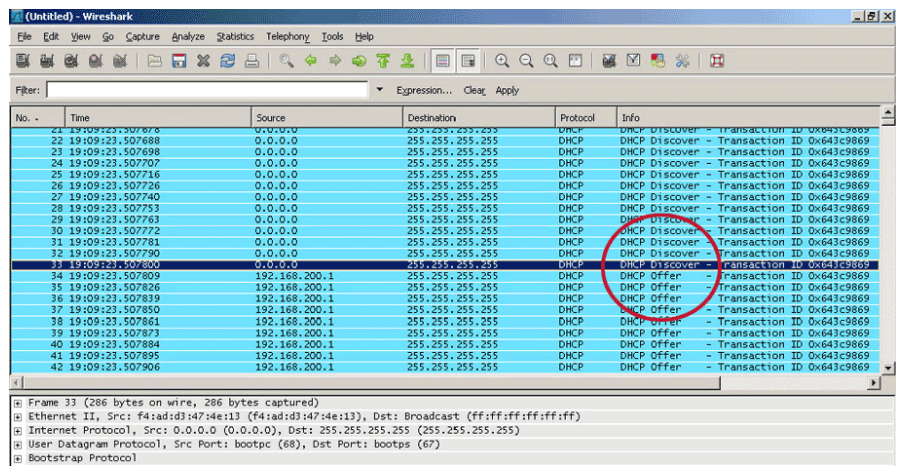
The above figure is an example of the result of using a tool that is called Yersinia to launch a DHCP attack against the DHCP server. The Yersinia tool is capable of generating DHCP DISCOVER requests using spoofed MAC address at a rapid rate to quickly exhaust the IP address pool on the DHCP server. All the DHCP clients of the victim network are starved of the DHCP resource. The attacker can then set up a rogue DHCP server on the network and perform man-in-the-middle attacks.

As shown in the Wireshark output above, a large amount of DHCP discover packets are being broadcasted out using different spoofed MAC addresses. The DHCP server (192.168.200.1) then responded with the DHCP offer packets until all the available IP addresses are exhausted.

IP Subnetting
To increase scalability, network administrators often need to divide networks (especially large networks) into subnetworks, or subnets. A subnet segments the hosts within the network. With proper network segmentation, even when attackers get in, their access is limited to only a segment of the network and not to the entire network. One very basic task that an analyst will need to perform is to determine which subnet that a given IP address belongs to. For example, when investigating the 10.1.1.36/24 IP address, one should be able to determine that this IP address belongs in the 10.1.1.0/24 subnet. Therefore, it is important for the security analyst to understand the purposes and functions of the subnets and their addressing schemes.

A subnet segments the hosts within the network. Without subnets, the network has a flat topology. A flat topology has a small routing table and relies on MAC addresses to deliver packets. MAC addresses have no hierarchical structure. As the network grows, the use of the network bandwidth becomes less efficient.

A company that occupies a three-story building might have a network that is divided by floors, with each floor divided into offices. Think of the building as the network, the floors as the three subnets, and the offices as the individual host addresses.

There are other disadvantages to a flat network. All devices share the same broadcast domain, and it is difficult to apply security policies because there are no boundaries between devices.

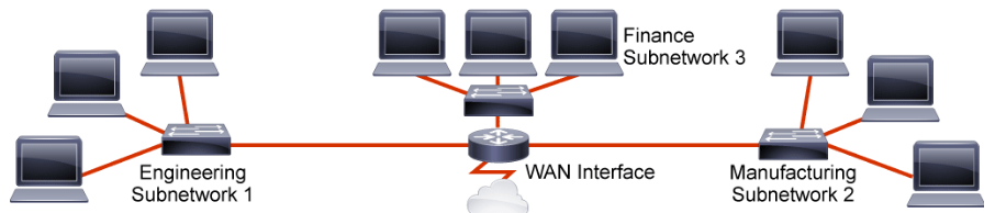
In multiple-network environments, each subnetwork may be connected to the Internet by a single router. This figure shows one router connecting multiple subnetworks to the Internet. The details of the internal network environment and how the network is divided into multiple subnetworks are inconsequential to other IP networks.

The advantages of subnetting a network are as follows:

Smaller networks are easier to manage and map to geographical or functional requirements.

Contain the broadcast traffic to the individual subnets to improve performance.

More easily apply network security measures at the interconnections between subnets than within a large single network.

Subnet Masks
The IP addressing that is used in the flat network must be modified to accommodate the required segmentation. A subnet mask identifies the network-significant portion of an IP address. The network-significant portion of an IP address is simply the part that identifies the network that the host device is on. This part is called the network address and defines every subnetwork. The use of segmentation is important for the routing operation to be efficient.

A subnet mask:

Defines the number of bits that represent the network and subnet part of the address

Is used by end systems to identify the destination IP address as either local or remote

Is used by Layer 3 devices to determine network path

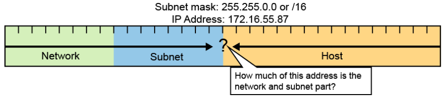
How do you know how many bits represent the network portion of the address and how many bits represent the host portion? When you express an IPv4 network address, you add a prefix length to the network address. The prefix length is the number of bits in the address that give the network portion. For example, in 172.16.55.87 /20, /20 is the prefix length. It tells you that the first 20 bits are the network address, leaving the remaining 12 bits as the host portion. The entity that is used to specify the network portion of an IPv4 address to the network devices is called the subnet mask. The subnet mask consists of 32 bits, just as the address does, and uses 1s and 0s to indicate which bits of the address are network bits and which bits are host bits. You express the subnet mask in the same dotted decimal format as the IPv4 address. The subnet mask is created by placing a binary 1 in each bit position that represents the network portion and placing a binary 0 in each bit position that represents the host portion. Both the network and host portion of the subnet mask must be continuous. A /20 prefix is expressed as a subnet mask of 255.255.240.0 (11111111.11111111.11110000.00000000). The remaining bits (low order) of the subnet mask are zeroes, indicating the host address within the network.

The subnet mask is configured on a host with its IPv4 address to help the host determine the network portion of that address. The host makes this determination by logically ANDing the binary bits of its IPv4 address with the binary bits of the subnet mask.

Networks are not always assigned the same prefix. Depending on the number of hosts on the network, the prefix that is assigned may be different. Having a different prefix number changes the host range and broadcast address for each network.

For example, look at the host 10.1.20.70/26:

Address:
- 10.1.20.70
- 00001010.00000001.00010100.01000110

Subnet mask:
- 255.255.255.192
- 11111111.11111111.11111111.11000000

Network address:
- 10.1.20.64
- 00001010.00000001.00010100.01000000

Variable-Length Subnet Masking
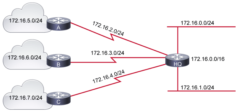
The figure below illustrates a network that uses fixed-length prefixes to address various segments. Address space is wasted because large subnets are used for addressing the WAN interfaces which are simply point-to-point segments. The three WAN segments only require the use of two host addresses, yet a subnet containing 254 hosts has been assigned to each WAN segment, wasting lots of usable IP addressing space.

VLSM affords the options of including more than one subnet mask within a network and of subnetting an already subnetted network address.

Network using VLSM:

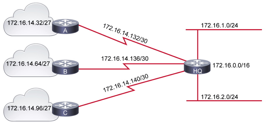
The subnet 172.16.14.0/24 is divided into smaller subnets

One subnet has a subnet mask /27.

Further subnetting of one of the unused /27 subnets into /30 subnets.

VLSM offers these benefits:

More efficient use of IP addresses: Without the use of VLSM, companies must implement a single subnet mask within an entire Class A, B, or C network number.

- For example, consider the 172.16.0.0/16 network address that is divided into subnetworks using /24 masking. One of the subnetworks in this range, 172.16.14.0/24, is further divided into smaller subnetworks using /27 masking. These smaller subnetworks range from 172.16.14.0/27, 172.16.14.32/27, 172.16.14.64/27, and so on to 172.16.14.224/27.

- In the figure, one of these smaller subnets, 172.16.14.128/27, is further divided using the /30 prefix, which creates subnets with only two hosts, to be used on the WAN links. The /30 subnets range from 172.16.14.128/30 to 172.16.14.156/30. The WAN links used the 172.16.14.132/30, 172.16.14.136/30, and 172.16.14.140/30 subnets out of the range.

Better-defined network hierarchical levels: VLSM allows more hierarchical levels within an addressing plan, which enables easier aggregation of network addresses. For example, in the figure, subnet 172.16.14.0/24 describes all the addresses that are further subnets of 172.16.14.0, including addresses from subnet 172.16.14.0/27 to subnet 172.16.14.128/30, and so on.

Hubs, Bridges, and Layer 2 Switches
LANs can vary widely in size. A LAN may consist of only two computers in a home office or small business, or it may include hundreds of computers in a large corporate office spanning a single or multiple buildings.

When you connect three or more devices together, you need a dedicated network device to enable communication between hosts. Network devices, such as the hubs, bridges, and switches, form the aggregation point for LANs. These devices enable communication between hosts by connecting them to the other segments of the network. A basic understanding of how these devices operate will help a security analyst investigate any malicious or suspicious activity from the logs that the devices generate.

A hub is a multiport repeater that takes an electronic signal that has been received from a device on one of its ports, magnifies the signal, and re-transmits that signal out all other ports on the hub, except for the original incoming port. Any traffic that comes into a hub or repeater port is sent out or repeated to all other ports. All ports on the hub share both a single collision domain and a single broadcast domain as the hub or repeater operates at the physical layer of the OSI model.

A collision domain, which is common in early versions of Ethernet, is a section of a network that is connected by a shared medium where data packets sent from one device will be heard by all other devices on the segment.

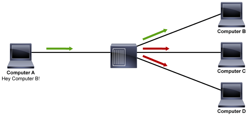
In the figure above, Computer A sends the message to Computer B through the hub. The hub, in addition to sending the message to the port where Computer B is connected, also sends the message out to the ports where Computer C and Computer D are connected, with no regard for where the actual destination host is connected to the hub. The bandwidth for the Computer C and Computer D are affected when Computer A and Computer B are communicating. Because everyone that is connected in this network can hear anyone’s message, you can use sniffing tools to easily eavesdrop on the network, which can also be a major security concern.

Whenever a packet is received on a port, the hub has no memory to store any data and the packet has to be transmitted. Hubs can run only in half-duplex mode where it can provide communication in both directions, but only one direction at a time. A network collision occurs when more than one device attempts to send a packet on a network segment at the same time.

To avoid the collision, devices in the Ethernet segment participate in the CSMA/CD (Carrier Sense Multiple Access with Collision Detection). This method uses a carrier sensing scheme in which a transmitting data station detects other signals on the wire and they won’t send their frame if someone else is using the wire. Simultaneous transmission still takes place and collision can happen. With the collision detection mechanism, the transmitting device stops transmitting the frame and transmits a jam signal when the collision is detected. Then the transmitting device waits for a random time interval, recognizing the need to retransmit before trying to resend the frame.

As the number of devices increase in hub-based environments, the problem gets much worse because of the nature of the half-duplex communication. Too many collisions and retransmissions occur which can lead to excessive LAN traffic congestion.

Traffic Flow: Hub vs. Bridge

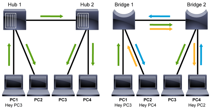
The left side of the diagram above shows the packet flow when the hosts are connected to the hub. All the devices must compete for the same bandwidth due to the half-duplex nature. So, when PC1 sends a message to the PC3, no other communications can happen between the devices in the network.

The right side of the diagram shows the packet flow when the hosts are connected to a bridge. In this example, review the simultaneous data flow, where PC1 sends traffic to PC3, PC2 sends traffic to PC4, and PC4 sends traffic to PC2. Ethernet bridges selectively forward individual frames from a receiving port to the port where the destination node is connected. This selective forwarding process can be thought of as establishing a momentary point-to-point connection between the transmitting and receiving nodes. The connection is made only long enough to forward a single frame. During this instance, the two nodes have a full-bandwidth connection between them and represent a logical point-to-point connection.

Need for Switches
Bridges and switches operate at the data link layer of the OSI model and use data link MAC addresses to differentiate between hosts that are connected to their ports. Although bridges preceded switches, these devices function in a similar way. These devices learn which ports lead to which host MAC addresses by monitoring the source MAC addresses in the Ethernet headers on frames that arrive on their switch ports. The port to MAC address mappings are stored in MAC address tables. The MAC address tables are commonly called CAM tables because many switches use CAM (a special type of technology) to store the MAC address tables.

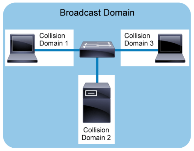
The figure above shows that the switch and each of its switch ports is connected to a single PC or a server. Switches are really multi-port bridges. Bridges perform the bridging logic that was usually implemented in software. In contrast, switches perform the Layer 2 switching in hardware. Today, it is common to use switches to divide a network into segments and reduce the number of devices that compete for bandwidth. Each new segment, then, results in a new collision domain. More bandwidth is available to the devices on a segment, and collisions in one collision domain do not interfere with the working of the other segments.

In the figure, each switch port represents a unique collision domain. All the ports on the switch fall under a single broadcast domain.

A broadcast domain is a logical division of a computer network, in which all nodes can reach each other by broadcast at the data link layer. Filtering frames by the MAC address of the switch does not extend to filtering broadcast frames. By their nature, broadcast frames must be forwarded. Therefore, all ports on a switch form a single broadcast domain. It takes a Layer 3 entity, such as a router, to terminate a Layer 2 broadcast domain.

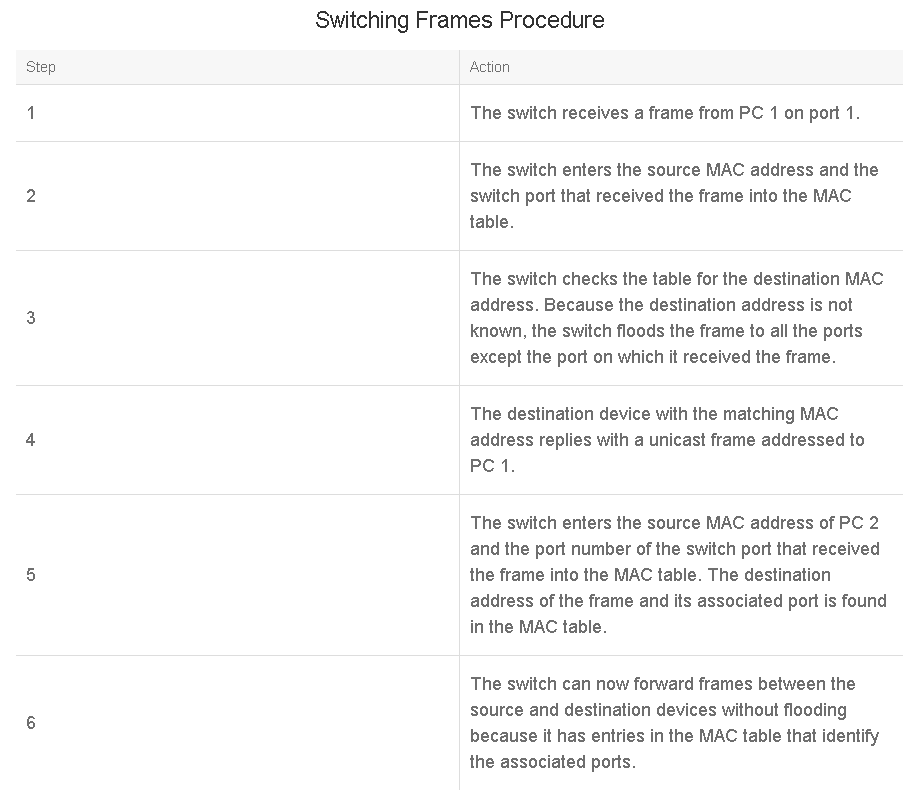
Switching Operations
Understanding switching operations will help analysts understand adversary operations against the Layer 2 devices in the network. For example, if an attacker can exhaust the switch’s MAC address table, the attacker can turn the switch into a hub. Therefore, analysts must understand the content of the MAC address table and how the information in the MAC address table is learned.

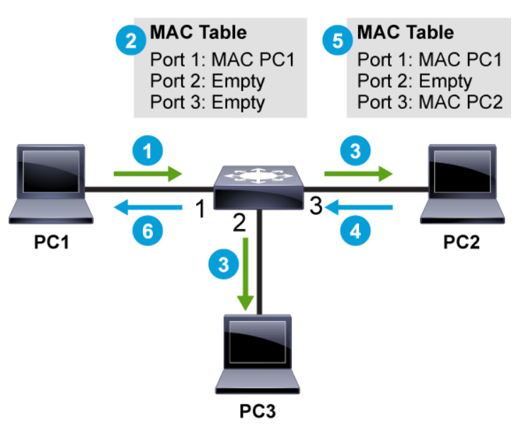
The switch builds and maintains a table, called a CAM table, that matches a destination MAC address with the port that is used to connect to a node. For each incoming frame, the destination MAC address in the frame header is compared to the list of addresses in the CAM table. Switches then use MAC addresses as they decide whether to filter, forward, or flood frames.

The switch creates and maintains a table using the source MAC addresses of incoming frames and the port number through which the frame entered the switch. When an address is not known, a switch learns the network topology by analyzing the source address of incoming frames from all the attached networks.

If a switch receives a frame that is destined for a MAC address that is in its MAC address table, then that frame is only forwarded out of the appropriate port leading to that MAC address. This conserves bandwidth on all the other ports on the switch. If the switch receives a frame that is destined for a MAC address that is not in its MAC address table, it floods the frame out of all ports, except for the port where the frame was received. If the destination replies to the source, the switch will be able to learn the new MAC address based on the source MAC address in the Ethernet header of the reply.

The table describes the switching process:

Look at a tool that an attacker uses to falsely generate MAC addresses to fill up the CAM table.

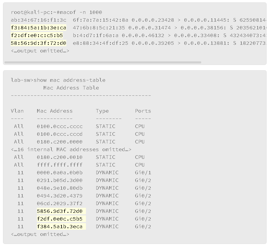
The above output is an example of the MAC flooding attack against the switch’s MAC address table using a Linux attack tool called macof, which is mainly used to flood the switch on a local network with MAC addresses. There is a limited amount of space available in the switch’s MAC address table. If the space is exhausted, the switch cannot learn new addresses. Traffic that is destined for an unknown MAC address will be flooded out all the ports, turning the switch into hub, which can lead to information disclosure if the attacker captured flooded frames and obtain sensitive information. It can also lead to a denial of service as network performance can be affected.

As shown in the show mac address-table output, many MAC addresses are learned on the port Gi0/2. Highlighted MAC addresses on the output are generated by the macof tool from the Linux system. The injection of the MAC addresses using the macof tool is very quick and can quickly fill the MAC address table of the switch.

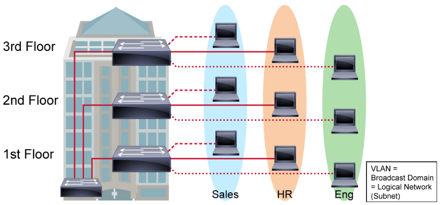
VLANs and Trunks
A VLAN is a logical broadcast domain that can span multiple physical LAN segments. Within the switched internetwork, VLANs provide segmentation and organizational flexibility. A VLAN structure can be designed to group stations that are segmented logically by functions, project teams, and applications, without regard to the physical location of the users.

When investigating Layer 2 attacks, an analyst should understand the functions of VLANs.

Within the switched internetwork, VLANs provide segmentation and organizational flexibility. Using VLAN technology, you can group switch ports and their connected users into logically defined communities. Examples might include the following:

Co-workers in the same department

A cross-functional product team

Diverse user groups sharing the same network application

A VLAN is a group of devices on one or more LANs that are configured to communicate as if they were attached to the same wire, when in fact they are located on several different LAN segments. Because VLANs are based on logical instead of physical connections, they are extremely flexible.

VLANs define broadcast domains in a Layer 2 network. A broadcast domain is the set of all devices that will receive broadcast frames originating from any device within the set. Broadcast domains are typically bounded by routers because routers do not forward broadcast frames. Layer 2 switches create broadcast domains that are based on the configuration of the switch. Switches are multiport bridges that allow you to create multiple broadcast domains. Each broadcast domain is like a distinct virtual bridge within a switch.

Each VLAN created in the switch defines a new broadcast domain. Traffic cannot pass directly to another VLAN (between broadcast domains) within the switch or between two switches. To interconnect two different VLANs, you must use routers or Layer 3 switches.

You can assign each switch port to only one VLAN, adding a layer of security. Ports in a VLAN share broadcast, but ports in different VLANs do not share broadcasts. Containing broadcasts within a VLAN improves the overall performance of the network by limiting the ability of broadcast traffic to span network segments.

A VLAN can exist on a single switch or span multiple switches. VLANs can include stations in a single building or multiple-building infrastructures.

A port normally carries only the traffic for the single VLAN to which it belongs. For a VLAN to span across multiple switches, a trunk must be configured to connect the two switches together. A trunk can carry traffic for multiple VLANs as shown in the following figure. A trunk allows multiple VLANs to share the port connection.

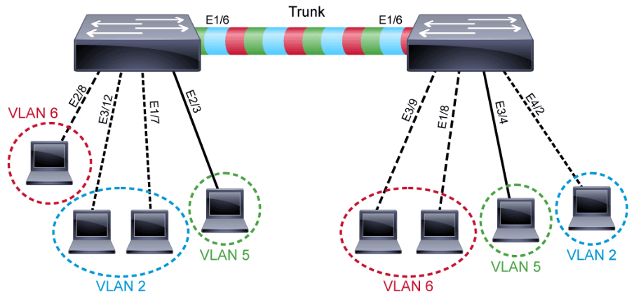
A trunk is a point-to-point link between an Ethernet switch interface and another networking device, such as a router or a switch. Ethernet trunks carry the traffic of multiple VLANs over a single link and allow you to extend VLANs across an entire network. A trunk does not belong to a specific VLAN. Rather, it is a conduit for VLANs between switches and routers.

You can configure an interface as trunking or nontrunking. If you configure an interface as trunking, it supports various trunking modes. Also, a trunk interface can be configured to negotiate trunking with neighboring interfaces.

A special trunking protocol, IEEE 802.1Q is used to carry multiple VLANs over a single link between two devices. A trunk could also be used between a network device and a server or another device that is equipped with an appropriate 802.1Q-capable NIC.

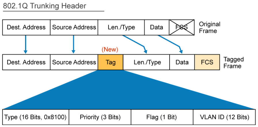
When Ethernet frames are placed on a trunk, they need additional information about the VLANs to which they belong. They get this information by using the 802.1Q encapsulation header. 802.1Q uses an internal tagging mechanism that inserts a 4-byte tag field into the original Ethernet frame between the Source Address and Type or Length fields. Because 802.1Q alters the frame, the trunking device recomputes the FCS on the modified frame. It is the responsibility of the Ethernet switch to look at the 4-byte tag field and determine where to deliver the frame.

By default, on a Cisco Catalyst switch, all configured VLANs are carried over a trunk interface. On an 802.1Q trunk port, there is one native VLAN, which is untagged (by default, VLAN 1). All other VLANs are tagged with a VLAN ID.

Spanning Tree Protocols
A topology with loops can be useful and potentially harmful. A loop implies the existence of multiple paths through the internetwork, and a network with multiple paths from source to destination can increase overall network fault tolerance through improved topological flexibility.

STP is a Layer 2 protocol that runs on bridges and switches. Without STP, the switched (or bridged) network will fail when there are redundant paths in the switched (or bridged) network. To understand the attacks that can be carried out against STP, analysts should understand STP.

The STP was originally developed by Digital Equipment Corporation, a key Ethernet vendor, to preserve the benefits of loops while eliminating their problems. Digital’s algorithm later was revised by the IEEE 802 committee and was published in the IEEE 802.1D specification.

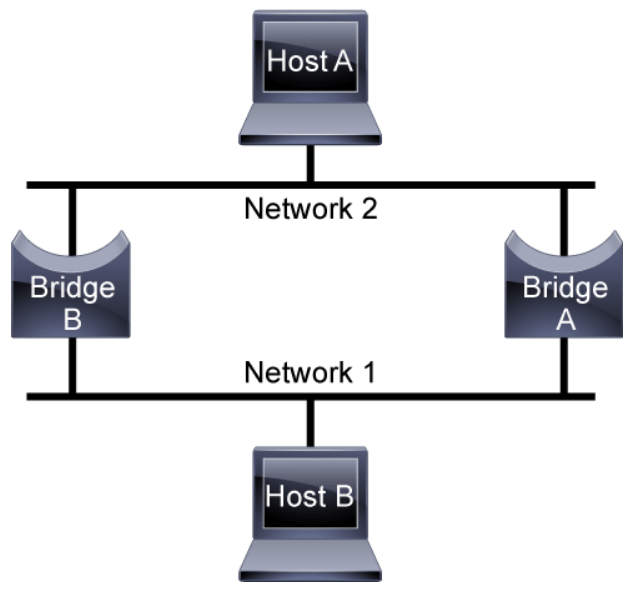
The following sequence of events occurs when an application on Host A communicates with Host B which causes a broadcast storm which will disrupt all the traffic on the switched network:

Host A sends a frame to Host B.

Bridge A learns that MAC address of Host A is located on its top port.

Bridge A looks up the MAC address of Host B; if no match is found (since Host B hasn't talked yet), Bridge A sends out the frame on its bottom port (known as flooding).

Bridge B also receives the frame on its top link and updates its MAC address table that Host A is located on its top port.

A split-second later, Bridge B receives the exact same frame on its bottom link; this time, it causes a new update to its MAC address table, which is known as a race condition—whichever MAC address arrives first wins the race and gets installed in the MAC address table.

Bridge B looks up the MAC address of Host B; if no match is found (since Host B has not talked yet), Bridge B sends out the frame on either its top or bottom port, depending on the outcome of the race condition described in Step 5.

Bridge A and Host B both receive the frame; however, this frame causes Bridge A to again update its MAC address table.

Return to Step 3 and loop forever. Even if Host B talks, nothing changes because both switches constantly update their MAC address tables with incorrect information (because of the never-ending loop). There is no TTL field in Ethernet headers to eventually stop the frame from looping.

In addition to basic connectivity problems, the proliferation of broadcast messages in networks with loops represents a potentially serious network problem. Assume that Host A’s initial frame is a broadcast. Both bridges forward the frames endlessly, using all available network bandwidth and blocking the transmission of other packets on both segments.

The spanning-tree protocol designates a loop-free subset of the network’s topology by placing those bridge ports that, if active, would create loops into a standby (blocking) condition. Blocking bridge ports can be activated in the event of a primary link failure, providing a new path through the internetwork.

To prevent loops in a network, a reference point for the network must first be defined. This reference point is called a root bridge. A root bridge is the logical center of the spanning tree topology. All paths that are not needed to reach the root bridge from anywhere in the network are placed in STP blocking mode. The spanning-tree protocol calculation occurs when the bridge is powered up and whenever a topology change is detected. The calculation requires communication between the spanning-tree bridges, which is accomplished using BPDUs.

Since the original creation of the IEEE 802.1D specification, many enhancements have been added to network devices to improve spanning-tree performance. Some of these enhancements were implemented to speed up STP performance (UplinkFast, BackboneFast, PortFast), and others are configured to increase security (BPDU guard, BPDU filter, root guard, loop guard). There are also other mechanisms that are not directly related to STP, but can be used to either complement STP operation (UDLD) or to replace it (FlexLinks).

Today, there are various flavors of STP, such as the IEEE specs (802.1D Common STP, 802.1w Rapid STP, 802.1s Multiple STP) or the proprietary vendor extensions. Each of these STP implementations functions in a similar fashion—typically differentiated by the amount of time that they need to recalculate an alternate topology (or converge) when there is a link failure, and the way that STP works with multiple VLANs.

Look at a sample MAC flap log message and explore it in more detail.


5d: %SW_MATM-4-MACFLAP_NOTIF: Host 0012.950a.9952 in vlan 10 is flapping between port Gi1/1 and port Gi1/2

This log information is a MAC flap notification message and tells that the MAC address of 0012.950a.9952 in VLAN 10 is flapping between ports G1/1 and G1/2 on the switch. There could be various reasons for this event being triggered.

For example, if there is an attacker on the port G1/2 trying to spoof the MAC address of the host on G1/1, then there is a possibility that the switch generated the log message. This type of event is not always triggered by an attacker. Sometimes, in a network with redundant links, due to misconfigurations or interface flaps, STP might toggle the redundant links, which also could have caused the MAC address flap.

In the scenario above, a security analyst can use their knowledge of STP to analyze the log information and narrow down the issue a lot faster, which can save time while identifying or correlating attacks on the network infrastructure.

Standalone (Autonomous) and Lightweight Access Points
Wireless networks are everywhere today; at home, in shopping malls, at coffee shops, at the airport, at the office, and so on. There are many attacks that can be launched against wireless networks. A very basic attack is where the attacker hosts a rogue wireless AP to lure victims to connect to it so that the attacker can capture the victim’s traffic. A rogue AP is an access point that has been installed on a secure network without explicit authorization from a system administrator. Understanding the concepts of autonomous and the lightweight access points will help the security analyst in their mission to secure these important yet vulnerable network resources.

A wireless AP is a wireless LAN networking hardware device that allows a Wi-Fi compliant device with a wireless network adaptor to connect to a wired network. The AP converts the radio frequency communications into digital signals and vice versa. The AP usually connects to a router via a wired Ethernet connection as a standalone device. The AP can also be an integral component of the router itself. A Wi-Fi hotspot is the physical location where Wi-Fi access to a wireless LAN is available.

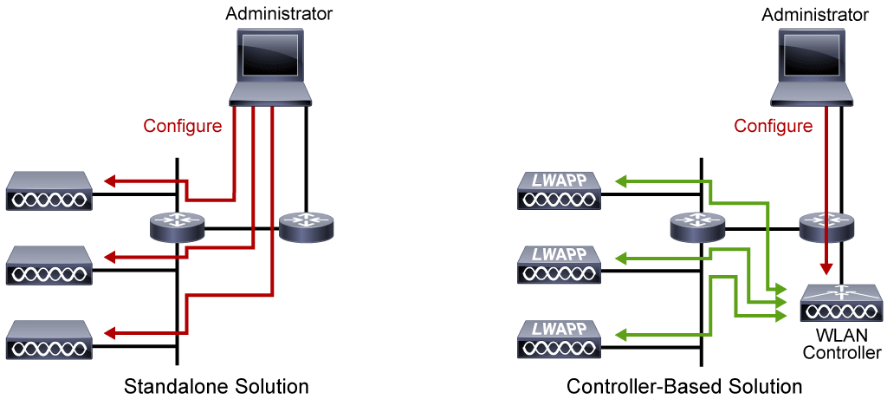
The figure shows two types of wireless access points. In the standalone solution, to make changes on the autonomous APs, the administrator must connect to each access point and perform the changes. In the controller-based solution, to make changes on the LWAPs (Lightweight Access Point), the administrator has to connect just to the WLAN controller and perform the changes.

Standalone (Autonomous) APs
Standalone (autonomous) APs can be configured one-by-one and offer complete functionality by themselves; they are well-adapted for very small deployments. Standalone APs support standalone network configurations, where all configuration settings are maintained locally. Each standalone AP can load its starting configuration independently, and still operate in a cohesive fashion on the network. The autonomous AP is equipped with both wired and wireless hardware so that wireless client associations can be terminated onto a wired connection locally at the AP. The APs and their data connections must be distributed across the coverage area and across the network.

Autonomous APs are self-contained, each offering one or more fully functional, standalone BSSs (Basic Service Set). BSS is wireless service that is provided by an AP to one or more associated clients. The AP serves as a single point of contact for every device that wants to use the BSS. It advertises the existence of the BSS so that devices can find it and try to join. To do that, the AP uses a unique BSSID (Basic Service Set Identifier) that is based on the AP’s own radio MAC address.

In addition, the AP advertises the wireless network with an SSID (Service Set Identifier), which is a text string containing a logical name. Think of the BSSID as a machine-readable name tag that uniquely identifies the BSS ambassador (the AP), and the SSID as a non-unique, human-readable name tag that identifies the wireless service.

Autonomous APs are also a natural extension of a switched network, connecting wireless SSIDs to wired VLANs at the access layer.

The above figure shows the basic architecture of an autonomous AP and focuses on just one AP and its connections. The wireless network consists of two SSIDs: WLAN 100 and WLAN 200, which correspond to wired VLANs 100 and 200, respectively. The VLANs must be trunked from the distribution layer switch (where routing commonly takes place) to the access layer, where they are extended further over a trunk link to the AP.

Wireless users join using the SSIDs and the data has to travel only through the AP to reach the network on the other side. An autonomous AP must also be configured with a management IP address (10.10.10.10 in the figure) so that you can remotely manage it. The management address is not normally part of any of the data VLANs, so a dedicated management VLAN (VLAN 10 in the figure) must be added to the trunk links to reach the AP.

Lightweight APs
There are some disadvantages in using the autonomous APs. As a network administrator, you are in charge of selecting and configuring the channel that is used by each autonomous AP and detecting and dealing with any rogue APs that might be interfering. You must also manage things such as the transmit power level to make sure that the wireless coverage is sufficient, does not overlap too much, and there are no coverage holes—even when an AP’s radio fails.

Managing wireless network security can also be difficult. Each autonomous AP handles its own security policies, with no central point of entry between the wireless and wired networks. That means there is no convenient place to monitor traffic for things such as intrusion detection and prevention, quality of service, bandwidth policing, and so on.

Early implementers of WLAN systems that used “fat” access points (autonomous or intelligent APs) found that the implementation and configuration of such APs was the equivalent of deploying and managing hundreds of individual firewalls, each requiring constant attention to ensure correct firmware, configuration, and safeguarding. Even worse, APs are often deployed in physically unsecured areas where theft of an AP could result in someone accessing its configuration to gain information to aid in some other form of malicious activity.

To overcome the limitations of distributed autonomous APs, many of the functions that are found within autonomous APs have to be shifted toward some central location.

LWAPs rely on a central WLC (Wireless LAN Controller) where the configuration is managed. LWAPs retrieve their configurations from a central WLC. They are called “lightweight” APs because most of the wireless LAN administration work is done by the central WLC.

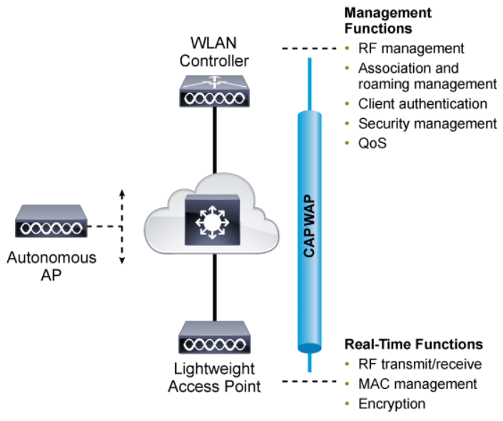
The above figure shows how most of the activities that are performed by an autonomous AP are broken up into two groups for the lightweight AP: management processes on the top and real-time processes on the bottom.

The real-time processes involve sending and receiving IEEE 802.11 frames, beacons, and probe messages. 802.11 data encryption is also handled in real time, on a per-packet basis. The AP must interact with wireless clients on some low level, which is known as the MAC layer. These functions must stay with the AP, closest to the clients.

The management functions are not integral to handling frames over the RF channels, but are things that should be centrally administered. Therefore, those functions are moved to a centrally located platform away from the AP.

The two devices must use a tunneling protocol between them, to carry 802.11-related messages and also client data. Lightweight AP and WLC can be located on the same VLAN or IP subnet, but they do not have to be. Instead, they can be located on two entirely different IP subnets in two entirely different locations.

The CAPWAP (Control and Provisioning of Wireless Access Points) tunneling protocol makes this possible by encapsulating the data between the LWAP and WLC within new IP packets. The tunneled data can then be switched or routed across the campus network.

Once CAPWAP tunnels are built from a WLC to one or more lightweight APs, the WLC can begin offering various additional functions such as the following:

Dynamic channel assignment

Transmit power optimization

Self-healing wireless coverage

Flexible client roaming

Dynamic client load balancing

Security management

Wireless intrusion protection system

Let’s explore sample log information that is related to AP in more detail.


Sat Sep 12 17:42:39 2015: 00:0b:85:51:5a:e0 Received CAPWAP DISCOVERY REQUEST from AP 00:0b:85:51:5a:e0 to ff:ff:ff:ff:ff:ff on port '1'
Sat Sep 12 17:42:39 2015: 00:0b:85:51:5a:e0 Successful transmission of CAPWAP Discovery-Response to AP 00:0b:85:51:5a:e0 on Port 1
Sat Sep 12 17:42:50 2015: 00:0b:85:51:5a:e0 Received CAPWAP JOIN REQUEST from AP 00:0b:85:51:5a:e0 to 00:0b:85:33:52:80 on port '1'
Sat Sep 12 17:42:50 2015: spamRadiusProcessResponse: AP Authorization failure for 00:0b:85:51:5a:e0

This log shows the LWAP that is trying to join the controller. Review the CAPWAP messages that are exchanged between the APs and the WLAN controller, and finally, the AP authorization failure message for the AP with the MAC address of 00:0b:85:51:5a:e0.

With the basic understanding of a CAPWAP tunnel and how it is built between the WLC and the LWAP, a security analyst can identify whether the request made by the LWAP is valid or not. As it is an LWAP, all the configurations will need be performed on the WLC. So, the security analyst can quickly check or suggest that the network administrator checks the WLC for the AP’s MAC address, 00:0b:85:51:5a:e0, and determine whether the AP is valid or a rogue AP that is trying to get into the network.

As part of their job role, the security analyst will often be required to narrow down an issue to a specific root cause. In this example, with the knowledge of APs, a security analyst is able to analyze the logs to identify or correlate attacks on the network, and plan or implement security measures efficiently.

Routers
Understanding how routers operate helps the security analyst better understand adversary operations that are taken against routers in the network and analyze output logs generated by these devices. For example, if an attacker can corrupt a router’s routing table, the attacker can redirect the victim’s traffic to the attacker. Therefore, the analyst needs to be able to understand the content of the router’s routing table and how that information is learned.

Routing is the process that routers, OSI network layer devices, use to forward data packets between networks or subnetworks. The routing process uses network routing tables, protocols, and algorithms to determine the most efficient path for forwarding an IP packet. Routers gather routing information and update other routers about changes in the network. Routers greatly expand the scalability of networks by terminating Layer 2 collisions and broadcast domains.

Routers are required to reach hosts that are not in the local network.

Routers use a routing table to route between networks.

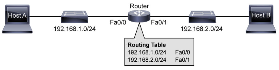
While switches switch data frames between segments to enable communication within a single network, routers are required to reach hosts that are not in the local LAN. Routers enable internetwork communication by placing the interface of each router in the network of the other routers. They use routing tables to route traffic between different networks.

Routers are devices that gather routing information from neighboring routers in the network. The routing information that is processed locally goes into the routing table. The routing table contains a list of all destinations that are known to the router and the information how to reach them. Routers have these two important functions:

Path determination: Routers must maintain their own routing tables and ensure that other routers know about changes in the network. Routers use a routing protocol to communicate network information to other routers. A routing protocol distributes the information from a local routing table on the router. Different protocols use different methods to populate the routing table. In the show ip route output in the figure, the first letter in each line of the routing table indicates which protocol was the source for the information (for example, O = OSPF). It is possible to statically populate routing tables by manually configuring static routes (S = static). However, statically populating routing tables does not scale well and leads to problems when the network topology changes. Static routes can also pose routing issues when the network design changes or when link outages occur.

Administrative distance is the feature that routers use to select the best path when there are two or more routes to the same destination network from two routing protocols. Routing protocols use different metrics to measure the distance and desirability of a path to a destination network. The metric calculation is done by the routing protocol. You can influence it by adjusting bandwidth, applying route-maps, or offset lists. Once the protocol is determined, the lowest metric is used to choose the appropriate route within the protocol when there are two or more routes to the same destination network. Administrative distance defines the reliability of a routing protocol. Each routing protocol is prioritized from most to least reliable (believable) with the help of an administrative distance value.

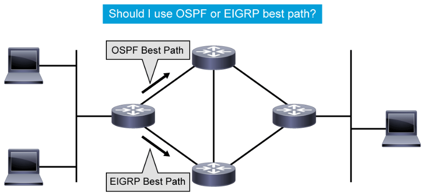
For example, in the figure, the router on the far left has two paths to the destination network on the far right. One of the paths is learned through a dynamic routing protocol, OSPF, and the other path is learned through EIGRP. Since EIGRP has a better (lower) administrative distance than OSPF, the router on the far left will use the EIGRP path and publish only the EIGRP path to the destination network in its routing table.

Packet forwarding: Routers use the routing table to determine where to forward packets. Routers forward packets through a network interface toward the destination network. Each line of the routing table indicates which network interface is used to forward a packet. The destination IP address in the packet defines the packet destination. Routers use their local routing table and compare the entries to the destination IP address of the packet. If there are multiple entries to the destination in the local routing table, the longer prefixes are always preferred over shorter ones when forwarding a packet. The result is a decision about which outgoing interface to use to send the packet out of the router. If routers do not have a matching entry in their routing tables, the packets are dropped and the router sends an ICMP message to the source address of the packet.

Types of Routes
Routers can learn about other networks via directly connected networks, static routes, dynamic routes, and default routes. This topic describes each of these types of routes.

The routing table can be populated by these methods:

Directly connected networks: This entry comes from having router interfaces that are directly attached to network segments. This method is the most certain method of populating a routing table. If the interface fails or is administratively shut down, the entry for that network is removed from the routing table. The administrative distance is 0 and therefore preempts all other entries for that destination network. Entries with the lowest administrative distance are the best, most-trusted sources.

Static routes: A system administrator manually enters static routes directly into the configuration of a router. The default administrative distance for a static route is 1; therefore, static routes will be included in the routing table unless there is a direct connection to that network. Static routes can be an effective method for small, simple networks that do not change frequently. For bigger or unstable networks, static routes are not a scalable solution.

Dynamic routes: The router learns dynamic routes automatically when a routing protocol is configured and a neighbor relationship to other routers is established. The information changes with changes in the network and updates constantly. Larger networks require the dynamic routing method because there are usually many addresses and constant changes. These changes require updates to routing tables across all routers in the network, or connectivity is lost.

Default routes: A default route is an optional entry that is used when no explicit path to a destination is found in the routing table. The default route can be manually inserted or it can be populated from a dynamic routing protocol.

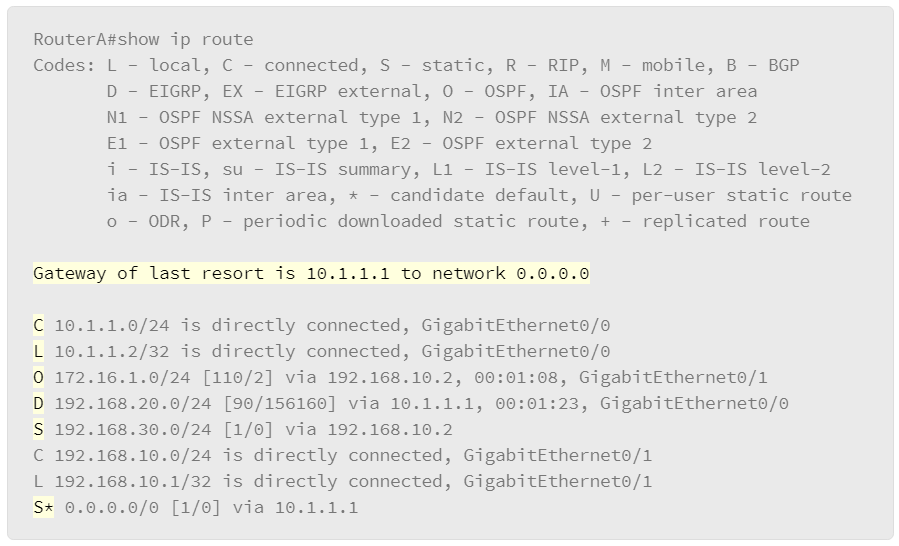
The figure displays the show ip route command, which is used to show the contents of the routing table in a router. The first part of the output explains the codes, presenting the letters and the associated source of the entries in the routing table.

C is for the directly connected networks.

L is for the local routes and indicates local interfaces within connected networks.

S is for the static routes. The letter S with an asterisk (*) indicates a static default route.

O is for the OSPF routing protocol.

D is for the EIGRP routing protocol. The letter D stands for DUAL, the update algorithm used by EIGRP.

Routing Protocols
Routing is one of the most important parts of the infrastructure that keeps a network running. Successful attacks against routers compromise the router itself, its peering sessions, or its routing information. Routing protocols are used by routers to learn routes and maintain routing tables. Having a basic knowledge of routing protocols will help the security analysts to identify potential attacks and take protective measures to prevent them.

The basic objective of routing protocols is to exchange network reachability information between routers and dynamically adapt to network changes. These protocols use routing algorithms to determine the optimal path between different segments in the network, and update routing tables with the best paths.

It is best practice to use one IP routing protocol throughout the enterprise, if possible. Often, one may manage network infrastructures where several routing protocols will coexist. One common example of when multiple routing protocols are used is when the organization needs to connects to two or more ISPs for Internet connectivity. In this scenario, the most commonly used protocol to exchange routes with the service provider is BGP (Border Gateway Protocol), while within the organization, OSPF (Open Shortest Path First) or EIGRP (Enhanced Interior Gateway Routing Protocol) are typically used.

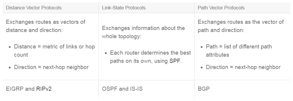
Several different possibilities exist when choosing the optimal routing protocol for your organization. There is no one optimal selection, so it is important that you understand the benefits and drawbacks of each protocol. The different routing protocols can be grouped in several ways. One option is to group them based on whether protocols operate within or between AS’s (Autonomous System).

An AS represents a collection of network devices under a common administrator. Typical examples of an AS are an internal network of an enterprise or a network infrastructure of an ISP.

Interior gateway protocols: IGPs are used within the organization, and exchange routes within an AS. They can support small, medium-sized, and large organizations, but their scalability has its limits. The protocols can offer very fast convergence, and basic functionality is easy to configure. The most commonly used IGPs in enterprises are EIGRP and OSPF. RIP (Routing Information Protocol) is also used, but rarely. IS-IS (Intermediate System-to-Intermediate System) is commonly found within the service provider internal network.

Exterior gateway protocols: EGPs take care of exchanging routes between different ASs. BGP is the only EGP that is used today. The main capability of BGP is to exchange a huge number of routes between different ASs that are part of the Internet.

Distance vector protocols: The distance vector routing approach determines the direction (vector) and distance (such as link metric or number of hops) to any link in the network. Distance vector protocols use routers as signposts along the path to the final destination. The only information that a router knows that about a remote network is the distance or metric to reach this network and which path or interface to use to get there. Distance vector routing protocols do not have an actual map of the network topology. While at first, the distance vector protocols supported only the periodic exchange of routing information, the two most commonly used distance vector protocols, EIGRP and RIPv2, use triggered updates to respond to topology changes.

Link-state protocols: The link-state approach, which uses the SPF algorithm, creates an abstract of the exact topology of the entire network, or at least of the partition in which the router is situated. Using an analogy of signposts, a link-state routing protocol is like having a complete map of the network topology. The signposts along the way from the source to the destination are not necessary because all link-state routers use an identical "map" of the network. A link-state router uses the link-state information to create a topology map and to select the best path to all destination networks in the topology. The OSPF and IS-IS protocols are examples of link-state routing protocols.

Path vector protocols: The path vector routing approach exchanges not only information about the existence of destination networks but also the path on how to reach the destination. Path information is used to determine the best paths and to prevent routing loops. Using an analogy of signposts, routers are not only familiar with the direction of the destination network but also with the specific path to the destination. The only widely used path vector protocol is BGP.

Routing protocols like BGP, IS-IS, OSPF, EIGRP, and RIPv2 provide a set of tools such as routing protocol authentication to help secure the routing infrastructure.

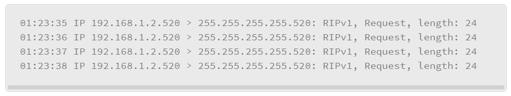
n the above sample log information, the IP address, 192.168.1.2 is sending the RIPv1 Request to the broadcast address, 255.255.255.255 on that segment. Routing Information Protocol (RIP) is one of the oldest distance-vector routing protocols which uses UDP 520 as its transport protocol. RIPv1 has no support for router authentication.

While analyzing the logs, if you see many messages like the one shown above, it is possible that an attacker is trying to perform the DoS attack to make the network resources unavailable. A malicious attacker can also spoof the source IP address and craft the same request query type as above, in order to form neighbors with nearby routers and get the complete routing information of the network. Once the network information is exposed, attackers may explore entire networks, and perform large-scale attacks.

The log message can also be generated when a legitimate router sends the RIPv1 request. With routing protocol knowledge, a security analyst can be aware of the circumstances when they get these types of log messages, and identify or correlate attacks faster on the networks.

Multilayer Switches
There are many different types of attacks that can occur at Layer 2 and Layer 3 in campus environments. It is important for analysts to understand how multilayer switches operate including how frame and packet forwarding take place on the switch. This knowledge will help when creating network defense mechanisms and can decrease the adversary’s likelihood of success with each subsequent intrusion attempt.

Multilayer switches (also known as Layer 3 switches) not only perform Layer 2 switching, but also forward frames that are based on Layer 3 and 4 information. Multilayer switches use ASIC (Application-Specific Integrated Circuit) hardware to perform header rewrites and forwarding.

The below figure shows a typical multilayer switch and the decision processes that must occur.

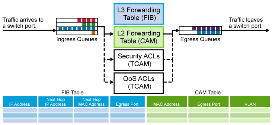
Packets arriving on a switch port are placed in the appropriate ingress queue, just as in a Layer 2 switch. Each packet is pulled off an ingress queue and inspected for both Layer 2 and Layer 3 destination addresses.

As with a Layer 2 switch, there are questions that need answers:

Where should I forward the frame?

Should I even forward the frame?

How should I forward the frame?

Decisions about these three questions are made as follows:

Layer 2 forwarding table: MAC addresses in the CAM (Content-Addressable Memory) table are used as indexes. If the frame encapsulates a Layer 3 packet that needs to be routed, the destination MAC address of the frame is that of the Layer 3 port on the multilayer switch.

Layer 3 forwarding table: The IP addresses in the FIB (Forwarding Information Base) table are used as indexes. The best match to the destination IP address is the Layer 3 next-hop address. The FIB also lists next-hop MAC addresses, the egress switch port, and the VLAN ID, so there is no need for additional lookup.

ACLs: The TCAM (Ternary Content-Addressable Memory) contains these ACLs (Access Control List). A single lookup is needed to decide whether the frame should be forwarded. TCAM is a specialized CAM designed for rapid table lookups.

QoS: Incoming frames can be classified according to QoS (Quality of Service) parameters. Traffic can then be prioritized and rate-limited. QoS decisions are also made by the TCAM in a single table lookup.

After CAM and TCAM table lookups are done, the packet is placed into an egress queue on the appropriate outbound Layer 3 switch port. The appropriate egress queue is determined by QoS, and more important packets are processed first.

On a Cisco Catalyst switch, a Layer 3 SVI (Switch Virtual Interface) can be configured for any VLAN that exists on the Layer 3 switch. The SVI provides Layer 3 processing for packets from all switch ports that are associated with that VLAN. Only one SVI can be associated with a VLAN. The SVI can be the default gateway for a VLAN so traffic can be routed between VLANs. The SVI also provides Layer 3 IP management connectivity to the switch.

Frame Rewrite
A multilayer switch, like a router, obtains next-hop destinations from the FIB table. Before forwarding the frame, it needs to rewrite certain parts of the frame.

When the frame arrives on the port, the destination MAC address of the frame belongs to the multilayer switch. After the switch processes the frame, the next-hop Layer 2 address must be put into the frame in place of the original destination address. The source MAC address of the frame is replaced with the MAC address that belongs to the multilayer switch. Also, the TTL is decreased by one, like with a router. The source and destination IP addresses stay the same.

When the frame arrives on the port, the switch does checksum calculation on the frame and IP packet to ensure that there was no frame or packet corruption during transit. Again, the frame and packet checksums are recalculated before being sent out of the switch.

CAM and TCAM Tables
Cisco Catalyst switches maintain CAM and TCAM tables. CAM is used in Layer 2 switching and TCAM is used in Layer 3 switching. Both tables are kept in fast memory so that processing of data is quick.

CAM:
- MAC address-to-port mappings
- Layer 2 forwarding decisions

TCAM:
- Found in multilayer switches and routers
- ACL, QoS, and other information for upper-layer processing - Switches can have multiple TCAMs to boost performance.

Multilayer switches forward frames and packets at wire speed by using ASIC hardware. Specific Layer 2 and Layer 3 components, such as learned MAC addresses or ACLs, are cached into the hardware. These tables are stored in CAM and TCAM.

CAM table: The CAM table is the primary table that is used to make Layer 2 forwarding decisions. The table is built by recording the source MAC address and inbound port of all incoming frames. When a frame arrives at the switch with a destination MAC address of an entry in the CAM table, the frame is forwarded out through only the port that is associated with that specific MAC address. If no exact match is found, the switch floods the packet out of all ports in the VLAN, except the incoming port.

TCAM table: The TCAM table stores ACL, QoS, and other information that is generally associated with upper-layer processing. Most switches have multiple TCAMs, such as one for inbound ACLs, one for outbound ACLs, one for QoS, and so on. Multiple TCAMs allow switches to perform different checks in parallel, thus shortening the packet-processing time. Cisco switches perform CAM and TCAM lookups in parallel. This behavior is the reason that Cisco switches do not suffer any performance degradation by enabling QoS or ACL processing.

NAT Fundamentals
NAT (Network Address Translation), defined in RFC 1631, operates in Layer 3 forwarding devices to provide address simplification and conservation. The most common use of NAT is to connect networks using private RFC 1918 network addresses to the public Internet. NAT translates the private addresses that are used in the internal network into public addresses that can be routed across the Internet. As part of this functionality, you can configure NAT to use only one address for the entire network to the outside world. Using only one address effectively hides the internal network, thus providing additional security. Understanding NAT operations helps the security analyst better understand adversary operations against the network devices and analyze output logs generated by these devices.

Multiple device types can be configured to perform NAT services. Although firewalls are most common, routers and some layer 3 switches are also capable of deploying this service.

Cisco defines the following list of NAT terms, which are illustrated in the figure below.

Inside local address: The IPv4 address that is assigned to a host on the inside network. The inside local address is likely to be one that falls within the RFC 1918 reserved private IPv4 address spaces.

Inside global address: A globally routable IPv4 address that represents one or more inside local IPv4 addresses to the outside world.

Outside local address: The IPv4 address of an outside host as it appears to the inside network. Not necessarily a public address, the outside local address is allocated from a routable address space.

Outside global address: The IPv4 address that is assigned to a host on the outside network by the host owner. The outside global address is allocated from a globally routable address or network space.

NAT offers the following benefits:

Eliminates the need to readdress all hosts that require external access, saving time and money.

Conserves addresses through application port-level multiplexing. With NAT, internal hosts can share a single registered IPv4 address for all external communications. In this type of configuration, relatively few external addresses are required to support many internal hosts, thus conserving IPv4 addresses.

The figure above illustrates a router that is translating the source address as the packet is forwarded from inside to outside, and reversing the translation on the reply that returns. The steps that are taken are as follows:

Host 10.10.10.11 sends a packet to host B.

The router receives the packet and checks its NAT table. It finds an entry to translate 10.10.10.11 to 203.0.113.2. If there was no entry in the table, the router would check the NAT rules to see if there is a rule specifying a dynamic translation. If there was such a rule, a new entry would be created.

The router replaces the inside local address 10.10.10.11 with the inside global address 203.0.113.2 and forwards the packet.

Host B receives the packet with 203.0.113.2 as the source address. When Host B replies, it specifies 203.0.113.2 as the destination address.

When the router receives the reply packet and checks its NAT table. It finds the entry that is associated with the inside global IPv4 address 203.0.113.2.

The router replaces the inside global address 203.0.113.2 with the inside local address 10.10.10.11 and forwards the packet.

NAT requirements will vary from situation to situation. The following deployment modes are available to address varying requirements:

Static NAT: This deployment choice maps an unregistered IPv4 address to a registered IPv4 address. One-to-one static NAT is particularly useful when a device must be accessible from outside the network. For example, static NAT is used when a server on a DMZ needs to be continuously reachable by the same predictable, translated address.

Dynamic NAT: This deployment choice maps an unregistered IPv4 address to a registered IPv4 address from a pool of registered IPv4 addresses which is useful for outbound client connections when you have fewer outside global IP addresses than inside local hosts.

Dynamic PAT: This deployment choice maps multiple unregistered IPv4 addresses to a single registered IP address by using the source port to distinguish between translations. That single IP address may be the IP address of the NAT device itself. Different systems may refer to dynamic PAT (Port Address Translation) using different terms. Examples include NAT overload, Hide NAT and Many to One NAT.

Static PAT: Imagine a network which has just one single public IP address. This IP address must be used by the firewall that connects the network to the Internet. It must also be used as the PAT address for all outbound connections. If this network must also support a DMZ server, then Static PAT can be used. For example, TCP port 80 may be reserved for PAT translation to the HTTP service on the DMZ server. Static PAT is sometimes called port forwarding.

Policy NAT: This deployment choice uses extended criteria, such as source addresses, destination addresses, and transport layer ports to specify the translation. For example, traffic that is destined to a particular partner network may be translated to a specific address using PAT while traffic destined elsewhere is translated using a dynamic NAT pool.

At this point, PAT is worthy of further consideration. One common variant of NAT is dynamic PAT. PAT is sometimes referred to as “NAT overload” or as “Hide NAT.” PAT allows you to translate multiple internal addresses into a few external addresses, or even a single external address, essentially allowing the internal addresses to share one external address.

PAT uses unique source port numbers on the inside global IPv4 address to distinguish between translations. Because the port number is encoded in 16 bits, the total number of internal addresses that NAT can translate into one external address is, theoretically, as many as 65,536. Some firewalls will also use destination IP address and port number to distinguish between translations. In this case, the same source port number can be used multiple times, increasing scalability even further. In either case, PAT allows for highly efficient use of address space for outbound sessions.

PAT allows multiple translations for individual hosts on the internal network. PAT also allows multiple hosts to use the same source port number. Most PAT implementations will try to preserve the inside local port number in the translation, and will randomly select a translation port if the original inside local port is in use by another translation.

Packet Filtering with ACLs
ACLs provide a basic level of security for network access. Without any ACLs configured on a router, all packets pass through the router and onto the network. ACLs can be configured on a router that is positioned between two parts of the network to control traffic that is entering or exiting a specific part of the internal network. An ACL on the router, for example, can allow one host to access a part of the network while, at the same time, preventing another host from accessing that same area.

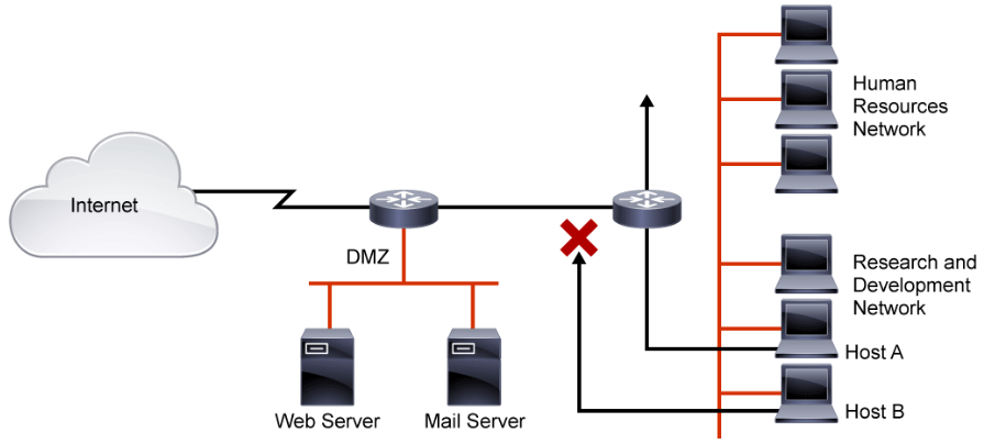
The ACL that is shown in the above figure allows host A to access the human resources network but prevents host B from accessing the human resources network.

To provide the security benefits of ACLs, at a minimum, configure ACLs at the network perimeter. This configuration provides a basic buffer from the outside network, or from a less controlled area of the network, onto network segments requiring more security. On these network edge routers, an ACL should be configured for each network protocol that is configured on the router interfaces.

Access Control List Example
The simplest type of firewall is a packet filter. As the name implies, packet filters look at individual packets in isolation. Based on the contents of the packet and the configured policy, they decide to permit or deny packets from entering or exiting the router interface. Packet filters generally have robust options for differentiating desirable and undesirable packets.

Common options include:

Source and destination IP addresses at the network layer.

Protocol differentiation at the transport layer: TCP, UDP, ICMP, OSPF, and so on

When the transport layer is TCP or UDP, source and destination ports can be specified.

When the transport layer is ICMP, types and codes can be specified.

When the traffic is TCP, the presence of the ACK bit or the RST bit can be verified. Under normal TCP connection flow, neither of these bits is ever set in the first packet of a new TCP connection.

Packet filtering is commonly implemented on Cisco IOS routers and switches. ACLs are used to classify packets. ACLs can be used for various functions on a Cisco IOS router. For example, they can be used to classify which packets are permitted into a priority queue. They can be used to classify which networks an OSPF process will advertise or which network advertisements an OSPF process will accept. They can be used to classify which packets will have their forwarding path specified by a policy-based route.

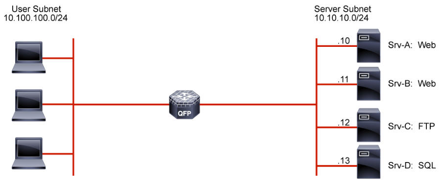
When an ACL is applied to an interface with the access-group command, it implements a packet filter. Consider the following ACL applied to the gi0/1 interface in the inbound direction regarding the topology that is depicted above:

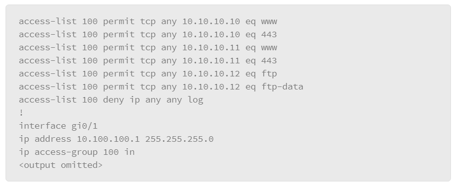
The ACL describes a policy of what is permitted and denied from the user subnet to the server subnet. To be effective, it can either be applied inbound on the interface connecting to the user subnet or it can be applied outbound to the interface connected to the server subnet. Some points of interest in this example include:

Clients on the user subnet are permitted to send packets to TCP ports 80 and 443 on the two web servers on the server subnet.

Clients on the user subnet are permitted to send packets to TCP ports 20 and 21 on the FTP server on the server subnet.

Standard FTP will function. Clients establish the control channel by connecting to port 21 on the FTP server. When the client requests a data transfer, it will obtain an ephemeral TCP port from its operating system and convey the appropriate port to the FTP server. The server will then open a data channel by connecting from TCP port 20 to the specified ephemeral port on the client. All packets that are sent from the client to the server that is associated with this data connection will be sent to TCP port 20.

Passive FTP will not function. Clients establish the control channel by connecting to port 21 on the FTP server. When the client requests a data transfer, it specifies the request as passive. The server application then requests an ephemeral port from its operating system and communicates the port to the client. The client then initiates the data channel by connecting to the ephemeral port on the server. This connection would not be allowed by the ACL as written, which is a single example of the difficulty packet filters have in handling protocols which use dynamically negotiated connections.

No connections are allowed from the user subnet to the SQL server. The SQL server is there to provide real time data to be presented by the web servers. Access to the data must be through the interface that is provided by the web servers. The SQL server is largely protected from the user subnet.

There is an explicit deny for all other packets as the last entry in the ACL. While this line is not required to deny all packets that were not matched by earlier entries, it does serve two purposes. First, hit counters are maintained for each line in the ACL. The administrator can use the show access-list 100 command to view the ACL and each entry’s hit count. Without the explicit deny, there would be no record of the number of packets that were denied by the ACL. Also, the explicit deny uses the log argument, which will cause the generation of syslog messages that are associated with the denies, which can facilitate central audit trails of rejected traffic. Unfortunately, ACL logging can be CPU intensive and can negatively affect other functions of the network device. It should therefore be used with discretion.


Note:
By default, there is an implicit deny ip any any entry at the end of every ACL. Anything that is not explicitly permitted is denied.

The ip access-group command is then used to apply the access list to an interface.

A primary focus of the security analysts is to investigate the ACL-related logs to identify or correlate attacks on the network. It would also be beneficial if a security analyst can assist the network administrators in troubleshooting or fixing certain issue by looking at the logs.


Mar 30 2016 11:41:48.681 EDT: %SEC-6-IPACCESSLOGP: list 185 denied tcp 172.16.1.92(59078) -> 192.168.2.1(80), 1 packet

Take a sample scenario where there is a complaint that the hosts on the 172.16.1.0/24 subnet cannot access the 192.168.2.1 Internal web server. For example, the above denied tcp log message indicates the connection from the source IP address, 172.16.1.92, to the destination IP address, 192.168.2.1 on TCP port 80, is denied.

With the basic knowledge of the access control list, a security analyst can quickly verify the ACL configuration regarding the 192.168.2.1 web server and the hosts on the 172.16.1.0/24 subnet. In this case, if it is not intended to deny the traffic from the hosts on the 172.16.1.0/24 subnet to the 192.168.2.1 web server on TCP port 80, and it looks to be a configuration issue, the security analyst can report the findings to the network administrator.

ACLs with the Established Option
A common requirement for access control is to allow TCP connections from the trusted network to a non-trusted network, and not allow TCP connections from a non-trusted network to the trusted network. Consider the figure below. A potential requirement is to allow hosts on NetA to initiate TCP connections to hosts on NetB, but not allow hosts on NetB to initiation connections to hosts on NetA.

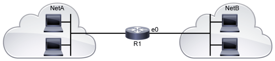
Stateless devices such as routers do not track the state of TCP connections and are challenged to meet this requirement. Cisco IOS extended ACLs provide the established keyword to approximate stateful behavior. The established keyword requires that either the ACK bit or the RST bit to be set in the TCP flags of a packet. Consider access-list 102 depicted below. It permits TCP packets from any source IP address to any destination IP address as long as either the TCP ACK bit or the TCP RST bit is set. This ACL is applied to R1 on interface Ethernet 0 in the inbound direction. Effectively, this will allow TCP connections originating from NetA and destined for NetB. At the same time it will deny TCP connections originating from NetB and destined for NetA.

Note that there are no ACL restrictions for packets originating from NetA and destined for NetB. The position and direction of the ACL only affects packets arriving from NetB. With no restrictions, a host on NetA can initiate a TCP connection to a host on NetB by sending a TCP SYN to start the three-way handshake. The reply packet from the host on NetB will have the TCP SYN and ACK bits set. This meets the established keyword criteria and is allowed. For the duration of this TCP connection, all packets from the host on NetB will have the ACK bit set, and hence the TCP connection is allowed. On the other hand, if a host on NetB attempts to initiate a TCP connection with a host on NetA, the first step of the three-way handshake is denied. This packet only has the SYN bit set. It does not meet the criteria of the established keyword.

It is important to understand that the established keyword does not imply stateful inspection. Each packet is considered independently with no consideration of TCP connection state. Consider this scenario. Access-list 102 does not permit ICMP traffic at all. Hence, hosts on NetB cannot use ICMP echo to perform a ping scan of NetA. But, given access-list 102, they can perform an ACK scan. A host on NetB could send crafted TCP packets with the ACK bit set to IP addresses on NetA. The active hosts on NetA will respond with TCP reset packets. Sending a TCP ACK and waiting for a TCP RST is fundamentally the same as sending an ICMP echo and waiting for an ICMP echo reply. A stateful packet filter would recognize that the crafted TCP ACK does not belong to an established TCP connection and would drop the packet.

This example is used to demonstrate the utility and the limitations of the established keyword available for TCP access control entries. In this scenario, the ACL is applied inbound on the interface that is connected to the untrusted network, but it could also be applied outbound on the interface that is connected to the trusted network.

Consider the following ACL regarding the topology that is depicted above:

In this scenario, the ACL would most likely be applied inbound on the interface that is connected to the untrusted network. Clients on the trusted network can establish the FTP control channel by connecting to TCP port 21 on the FTP server. The connection is initiated with a three-way handshake. The first packet, sent from the client to the server, only sets the SYN flag in the TCP header and it presents the clients initial sequence number. The server then responds with a packet that has both the SYN bit and the ACK bit set. The server presents its initial sequence number and it acknowledges the clients initial sequence number. The client then completes the three-way handshake with an ACK, acknowledging the server’s initial sequence number. Note that all packets from the server that are associated with this connection have the ACK bit set

FTP passive mode data channels can also establish. The FTP server will specify the ephemeral port to the client through the FTP control channel. The passive mode data channel is then opened with the client connecting to the server on the specified ephemeral port. As with the control channel, all packets from the server back to the client will have the ACK bit set.

However, standard mode FTP data channels will not function. The client will specify the ephemeral port to the server through the FTP control channel. The three-way handshake then begins with a TCP SYN sent from the FTP server to the client from source TCP port 20. This packet does not have the ACK bit set and hence the packet will be denied.

The last thing to point out in this scenario is an example of a limitation of relying on packet filters that reference the TCP flags in the TCP header of packets. Imagine the attacker in the topology wants to start reconnaissance by mapping out the IP addresses of hosts on the trusted side of the packet filter. Note that the ACL will not permit ping via ICMP echo requests. The attacker can, however, make clever use of an “ACK scan.” Instead of sending an ICMP echo request, the attacker can send a TCP packet with the ACK bit set to a destination address. Since the ACK bit is set, these packets will match the established keyword reference in the ACL and will be permitted. If there is a host present, that host will respond with a TCP reset (a TCP packet with the RST bit set) in response. The attacker can perform the same sort of reconnaissance as it could with ICMP ping. If a reset response is received, the IP address is active. If not, the IP address is not active.

[el7_blog] /dev/urandom

Cisco CCNA Cyber Ops SECFND 210-250, Section 2: Understanding the Network Infrastructure

[el7_blog]
/dev/urandom